What is the paper about?
Quantified uncertainty is helpful in many situations. In medical AI, for example, it tells you how (un-)certain you should be about a prediction and therefore can be an indicator of the confidence you should have. In simpler terms, there is a difference between “this thing might look like cancer, maybe you should have a look” and “OMG it’s cancer, rush to the hospital now!” and we should aim to know this difference.
However, uncertainty quantification is often hard in practice. The algorithms that provide uncertainty often use sampling strategies such as MCMC and scale badly with larger, more complex models. There are faster methods such as Variational Inference or Expectation Propagation that are faster but still have their own problems.
Therefore, our approach comes from a different angle. We use a “fast first, approximation quality second” strategy, where we look for approximations of which are known to be fast and then try to improve their approximation quality as much as possible. This is the basic premise for all research within my Ph.D. and this paper creates the foundations for it. We do this by investigating Generalized Linear Models (GLM) - arguable the simplest form of Bayesian Inference.
This post is a simple summary of the original paper. It is more visual and less mathy. If you want the full dose, check out the paper with accompanying code.
My personal take
Laplace Matching is really easy to use and the results are surprisingly good for such a simple idea. I would see it as a baseline, i.e. before you set up a complicated MCMC algorithm that runs for days, just test whether LM already gives you sufficiently accurate results. I’ll definitely use it more in the future and my current projects all build on it.
Background
There are three core techniques that underlie Laplace matching. If you properly understand all three, the rest of the paper is very simple.
Transformation of variable for PDFs
A probability density function is connected to a random variable. If you transform the random variable, e.g. you take its logarithm, then the corresponding pdf changes as well. Mathematically, this can be described with
\[\begin{aligned} p_Y(y) &= p_X(g^{-1}(y)) \left\vert \frac{d}{dy}(g^{-1}(y)) \right\vert \end{aligned}\]where \(g^{-1}\) describes the inverse function of \(g\), \(X\) is the original variable, \(Y\) the transformed variable and \(\left\vert \frac{d}{dy}(g^{-1}(y)) \right\vert\) the Jacobian of the inverse transformation.
Intuitively I find it easiest to think about the pdf in terms of a wire and the transformation as pulling or pushing the wire in different ways. If the transformation is linear, you push or pull everywhere equally, if it is non-linear you push or pull with different strength for different parts of the pdf.
I have written a separate blog post where I go into more detail on transformations of variables for pdfs.
Laplace approximations
Laplace approximations are a simple way to fit a Gaussian to a function - in our case a probability distribution. The mode of the function is taken as the mean of the Gaussian and the curvature at the mode is used to determine the variance of the Gaussian. Image is taken from this website.
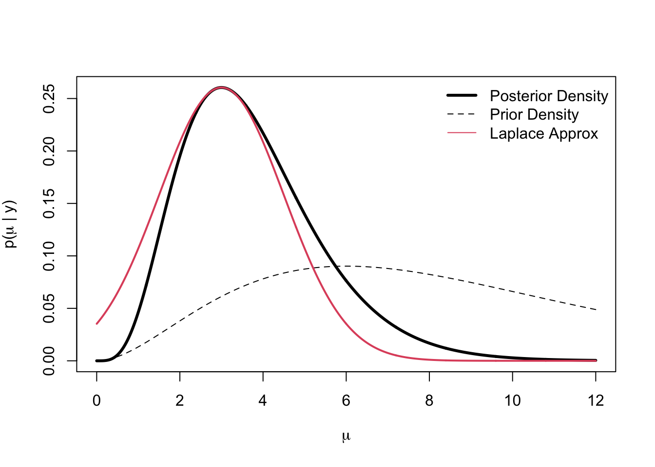
Most of the time it’s easy to get a Laplace approximation. You just have to differentiate the function once and set it to zero to get the mode. Then you have to differentiate it another time and invert the negative of the second derivative to get the variance.
If you want to understand the mathematical assumptions behind the Laplace approximation, I recommend checking out the respective section in the paper.
Exponential families
A pdf that can be written in the form
\[\begin{aligned}\label{EF} p(x) &= h(x)\cdot \exp\left(w^\top \phi(x) - \log Z(w) \right) \end{aligned}\]where
\[\begin{aligned} Z(w)&:= \int_{\mathbf{X}} h(x)\exp\left(w^\top \phi(x)\right) \,dx \end{aligned}\]is called an exponential family. \(\phi(x): \mathbb{X} \rightarrow \mathbb{R}^d\) are the sufficient statistics, \(w \in \mathcal{D} \subseteq \mathbb{R}^d\) the natural parameters with domain \(\mathcal{D}\), \(\log Z(w): \mathbb{R}^d \rightarrow \mathbb{R}\) is the (log) partition function (normalization constant), and \(h(x): \mathbb{X} \rightarrow \mathbb{R}_{+}\) the base measure.
Exponential families have a lot of interesting properties that I investigate in another post but for now we need to focus on only two.
Firstly, exponential families have sufficient statistics - they are the statistics of the data that tell you everything interesting about them, i.e. if you know the sufficient statistics another person with the same data is unable to tell more about the probability distribution than you are.
Secondly, exponential families usually have conjugate priors. This means that the posterior is described by the same probability distribution as the prior. The only thing that changes when observing new data are its parameters. If you observe the result of coin flips, for example, the Beta distribution can be updated by just changing its parameters \(\alpha\) and \(\beta\).
Laplace Matching
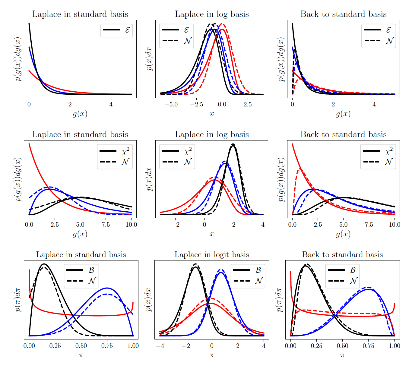
The motivation for Laplace Matching is very straightforward. Gaussians have nice properties, e.g. linear combinations of Gaussians are still Gaussians and they can be used for Gaussian Processes. To make everything Gaussian we could use Laplace approximations on non-Gaussian distributions. However, this leads to a couple of problems (left column): a) The Gaussian might be in the wrong domain. A Gaussian approximation to the Beta distribution is in \(\mathbb{R}\) while the Beta is only defined in probability space \(\mathbb{P}\). Therefore, parts of our approximation are undefined. b) For some parameters (red lines) there might not even be a Gaussian approximation because the second derivative is undefined. c) It might just not be a good approximation since, for example, a Gamma and a Gaussian just look quite different.
However, if we transform the variable (middle column) with a good transformation, exponential families suddenly look a lot more Gaussian and the Laplace approximation yields a better fit. Furthermore, the parameters for which we previously had no valid Laplace approximation (red lines) suddenly yield valid Laplace approximations in the different space. Even the domain is correct and the original distribution and its Laplace approximation are in the correct space.
To double-check if our new approximation is better, we transform it back to the original basis (right column). The approximations are better than the naive Laplace approximations on the left but they are still not perfect. The red line in the case of the Beta distribution, for example, goes to zero on the edges, where the originals go to infinity. This is the price we pay for being fast. Since we use a fixed transformation, the error we get is static, i.e. it doesn’t improve during runtime.
Laplace Matching is the process of finding the “right” transformation, e.g. it is on the correct domain, fast and as high-quality as possible. After the transformation has been found we have to develop the map from the parameters of the distribution \(\theta\) to \(\mu\) and \(\Sigma\) of the Gaussian approximation. Usually, this is done by computing the Laplace approximation in the chosen basis and inverting it. In some cases, e.g. the Dirichlet, the inversion is impossible and we have to use approximations for the inverse map.
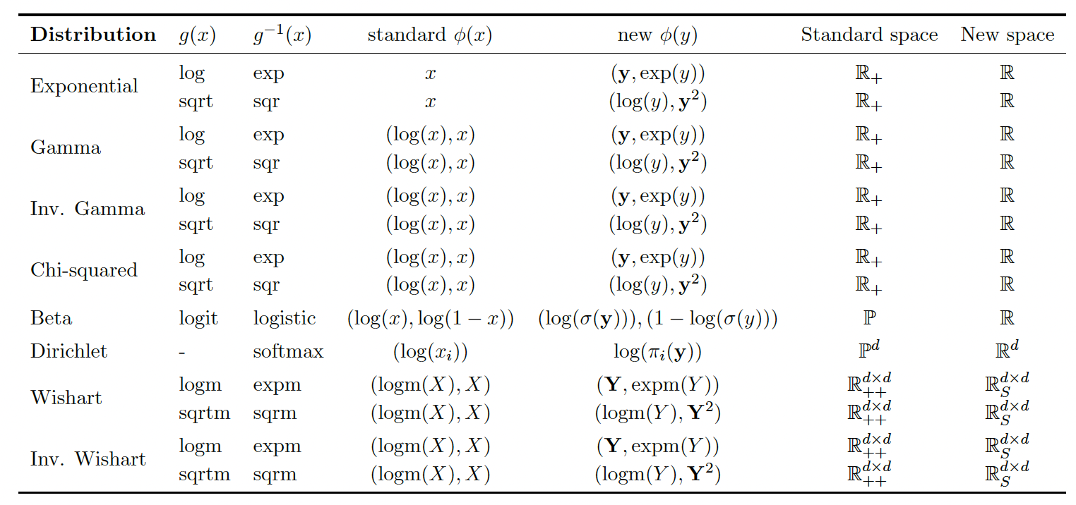
There is no clear optimal way of choosing the transformation since different transformation optimize different goals. However, we could show that the KL-divergence between the Gaussian and the exponential family distribution is minimized by moment matching, i.e. when the expected sufficient statistics are as similar as possible. This theoretical result still leaves some room for interpretation because the moments will never match perfectly. In the case of the Gamma distribution, for example, the original sufficient statistics of \([\log(x), x]\) can be transformed via the exponential function to be \([x, \exp(x)]\) or via the square to be \([\log(x), x^2]\). Both of these share one sufficient statistic with the Gaussian which has \([x, x^2]\). However, from a theoretical perspective, it’s not clear if either of them is optimal. Maybe even an interpolation between the two might be better. Therefore, we explored this empirically in the paper.
Laplace Matching can be applied to any exponential family. A core part of this work is to derive the transformations and respective mapping functions and their inverse for many commonly used distributions.
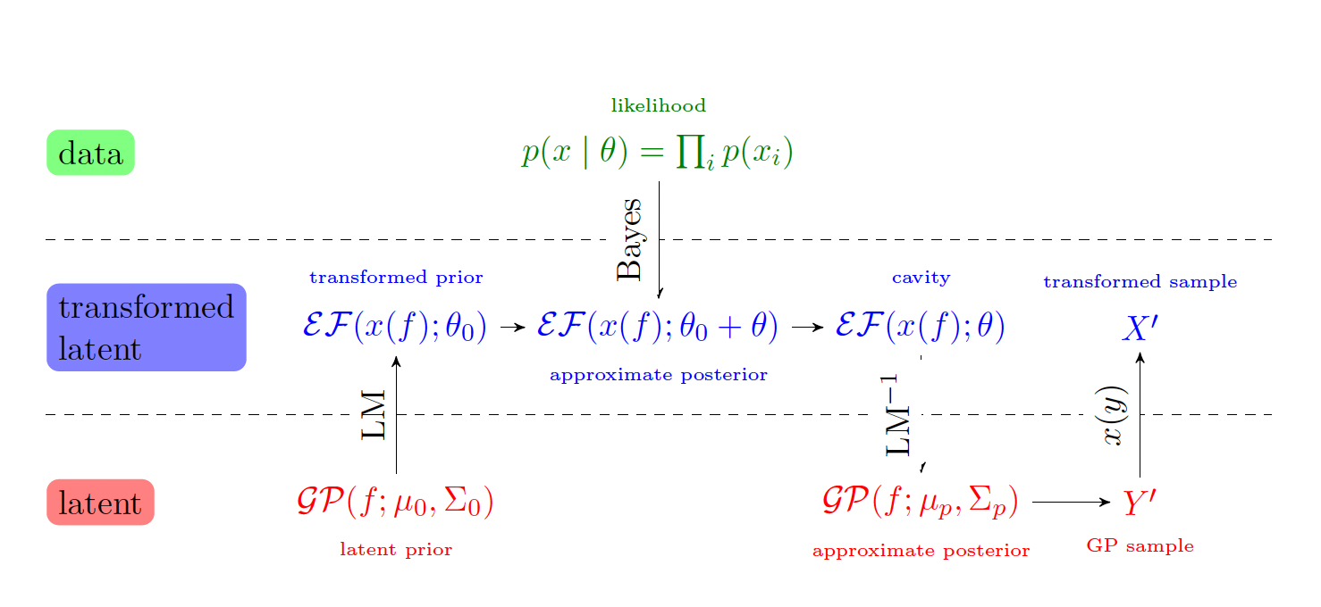
LM+GPs
An important use case of LM is in combination with Gaussian Processes (GP). The GP can include information through the kernel. Conventionally, this information is hard to incorporate in non-Gaussian models. LM is an easy fix for this. Therefore, adding a time component or making predictions on new data points becomes very easy for non-Gaussian data with LM+GP.
Experiments
We showcase LM+GP on three non-Gaussian datatypes.
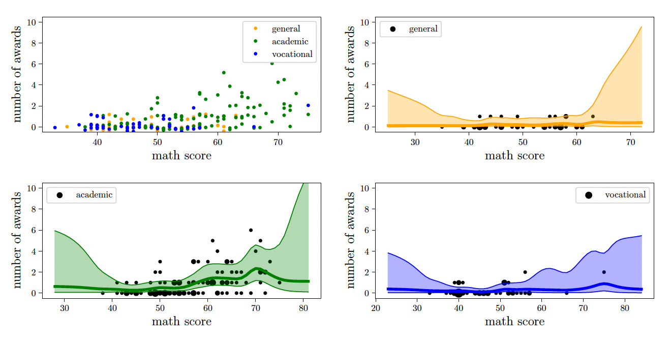
Poisson Toy Problem
We start with a simple toy problem with Poisson data. For every time step, we fit a marginal Gamma distribution through conjugacy. Then we use LM with the logarithm to get an estimate for \(\mu\) and \(\sigma\). On these, we fit a GP. For predictions outside of the training data, we can compute the marginal Gaussians of the GP, transform them back to the Gamma and plot confidence bounds. We could also draw samples and transform them back using the exponential. In any case, we get uncertainty estimates restricted to the positive domain for basically no additional cost.
Dirichlet Elections
For a slightly more complex problem, consider elections over time. Every election can be seen as a categorical sample of an underlying process (some might call this process “the will of the people”). Since elections only happen every couple of years, we have very little data at our hands. However, it might be interesting to see what the process looks like between elections or how future elections might look like under certain assumptions.
In our case, we look at the German federal elections after the second world war. We interpret every election count as a categorical variable to which the Dirichlet is a conjugate prior. This Dirichlet is now transformed to a Gaussian with LM and a GP is fit in the transformed space. Predictions are made by drawing sample functions from the GP and transforming them to probabilities via the softmax function.
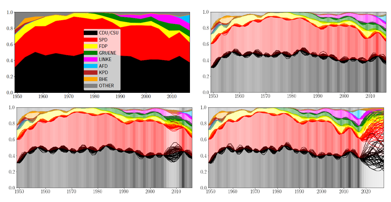
As you can see, LM+GP is able to interpolate between the data points and correctly quantify uncertainty, i.e. uncertainty is low at the training points and larger in between. LM+GP also correctly increases uncertainty when we remove one data point from the training data or predict into the future.
Inverse Wishart Currencies
Lastly, we look at Covariances. Especially when it comes to financial data it might be important to understand how Covariances change over time. To reduce risk in a portfolio, for example, you might want to buy anti-correlated stocks such as airlines and oil. When the oil price increases, airline stocks usually decrease in value. In the case of oil and airlines, the origin of the relationship is clear. For most stocks, however, it gets much more complicated. Therefore, we might be interested in how the covariance of stocks changes over time - in other words, we want to understand the underlying generative process. Empirical covariance matrices are positive semi-definite matrices and have an inverse Wishart conjugate prior distribution. Since we derived LM for the inverse Wishart, we are able to apply a GP to empirical covariance matrices.
In our case, we use currencies rather than stocks, but the principles stay the same.
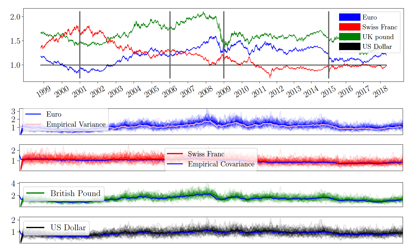
On top, you see the price of the currencies relative to the dollar. In four bottom columns you see samples of LM+GP and the true (co-)variance w.r.t. the euro. We see that the drawn samples all concentrate around the true function which indicates that the approximation loss of LM is very low.
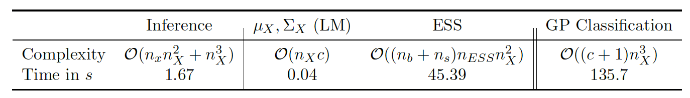
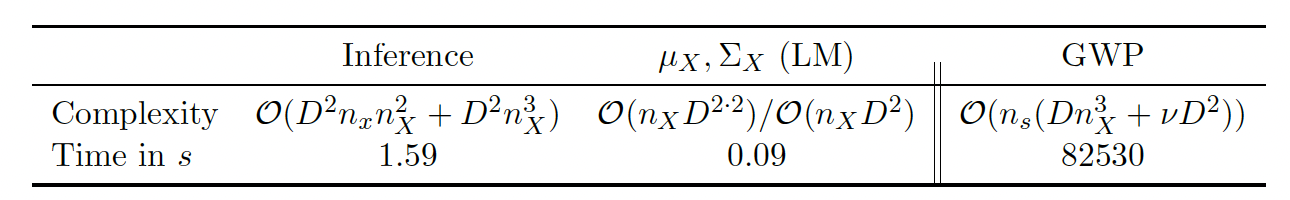
Timing and complexity
We are not the first to try and fit a GP to non-Gaussian data. In the case of categorical data, GP multi-class classification has existed for a long time and in the case of the Wishart, there is the Wishart process. While both of these approaches converge to the true solution eventually, they take very long to do so. LM, in comparison, is really fast and yields surprisingly accurate results.
Summary
The goal of my Ph.D. is to make Bayesian Inference fast. GLMs are an important foundation of Bayesian Inference and computations can take a long time, especially on non-Gaussian data. Laplace Matching is one way to do fast inference that is much faster than all alternatives. Laplace Matching has a fixed error, i.e. there are no iterations, hence no decrease in error during runtime. Empirically, we find this error to be quite low in all applications that we tried so far.
My personal take is that Laplace Matching is really easy to use and the results are surprisingly good for such a simple idea. I would see it as a baseline, i.e. before you set up a complicated MCMC algorithm that runs for days, just test whether LM already gives you sufficiently accurate results. I’ll definitely use it more in the future and my current projects all build on it.
One last note
If you want to get informed about new posts you can follow me on Twitter or subscribe to my mailing list.
If you have any feedback regarding anything (i.e. layout or opinions) please tell me in a constructive manner via your preferred means of communication.